Gender equality has been one of the hot topics for long time. There have been numerous stucdies, activities, and even law changes in order order to improve the gender equalities. Altghouh there is visible development in this regard, There is still more to do.
In this project I will analyze the gender equality or improvement in the movie industry. For that purpose, Bechdel Test will be employed. The Bechdel Test is comming from the idea that Alison Bechdel introduced in a comic strip and it has simple rules:
- At least two women
- The women need to talk to each other
- They need to talk to each other about something other than a man
The requirement of Bechdel Test is uncomplicated and asumming the majority of movies will be succesfull in terms of gender equality.
Looked for Couple of Insight
- Any Change of woman employment in movies over the years.
- The relationship of movie budget and woman employment if any.
- Female director imapct on the woman employment rate.
- Movie budget imapct on the woman employment rate.
- The woman employment rate impact on the movie revenue imapact.
# Importing Data From bechdeltest.com by their API
df = pd.read_json('http://bechdeltest.com/api/v1/getAllMovies')
df.head()
| rating | imdbid | year | id | title | |
|---|---|---|---|---|---|
| 0 | 0 | 3155794 | 1874 | 9602 | Passage de Venus |
| 1 | 0 | 14495706 | 1877 | 9804 | La Rosace Magique |
| 2 | 0 | 2221420 | 1878 | 9603 | Sallie Gardner at a Gallop |
| 3 | 0 | 12592084 | 1878 | 9806 | Le singe musicien |
| 4 | 0 | 7816420 | 1881 | 9816 | Athlete Swinging a Pick |
There are five features in data frame. Rating is the most I will work on because here it will be the main criteria to check if the movie pass the test or not. Rating less than 3 means failre while greater than 3 means pass.
Since the world does not have such a succes on gender equality in past let`s analyze data after 1970s.
df['rating'].value_counts()
3    5451
1    2085
0    1069
2     965
Name: rating, dtype: int64
data_bechdel = df[df['year']>=1970]
data_bechdel.head()
| rating | imdbid | year | id | title | |
|---|---|---|---|---|---|
| 1356 | 0 | 0065531 | 1970 | 255 | Le Cercle Rouge |
| 1357 | 3 | 0065466 | 1970 | 583 | Beyond the Valley of the Dolls |
| 1358 | 3 | 0065421 | 1970 | 1122 | AristoCats, The |
| 1359 | 1 | 0066327 | 1970 | 1726 | Santa Clause is Comin' to Town |
| 1360 | 1 | 0064806 | 1970 | 1932 | Phantom Tollbooth, The |
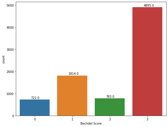
I am now going to rename the column ‘rating’ to ‘Bechdel Score’, to make things clearer for the rest of the analysis.
data_bechdel.rename(columns={'rating':'Bechdel Score'},inplace=True)
data_bechdel.head()
| Bechdel Score | imdbid | year | id | title | |
|---|---|---|---|---|---|
| 1356 | 0 | 0065531 | 1970 | 255 | Le Cercle Rouge |
| 1357 | 3 | 0065466 | 1970 | 583 | Beyond the Valley of the Dolls |
| 1358 | 3 | 0065421 | 1970 | 1122 | AristoCats, The |
| 1359 | 1 | 0066327 | 1970 | 1726 | Santa Clause is Comin' to Town |
| 1360 | 1 | 0064806 | 1970 | 1932 | Phantom Tollbooth, The |
Here I am going to convert the ‘year’ column into a datetime object to analyze data. easily.
data_bechdel['year'] = pd.to_datetime( data_bechdel['year'],format='%Y')
data_bechdel
| Bechdel Score | imdbid | year | id | title | |
|---|---|---|---|---|---|
| 1356 | 0 | 0065531 | 1970-01-01 | 255 | Le Cercle Rouge |
| 1357 | 3 | 0065466 | 1970-01-01 | 583 | Beyond the Valley of the Dolls |
| 1358 | 3 | 0065421 | 1970-01-01 | 1122 | AristoCats, The |
| 1359 | 1 | 0066327 | 1970-01-01 | 1726 | Santa Clause is Comin' to Town |
| 1360 | 1 | 0064806 | 1970-01-01 | 1932 | Phantom Tollbooth, The |
| ... | ... | ... | ... | ... | ... |
| 9565 | 1 | 13145534 | 2022-01-01 | 10370 | Incroyable mais vrai |
| 9566 | 2 | 10298810 | 2022-01-01 | 10371 | Lightyear |
| 9567 | 3 | 3513500 | 2022-01-01 | 10372 | Chip 'n Dale: Rescue Rangers |
| 9568 | 1 | 14169960 | 2022-01-01 | 10375 | All of Us Are Dead |
| 9569 | 3 | 15521050 | 2022-01-01 | 10382 | Love and Gelato |
8214 rows × 5 columns
Next, Bechdel Scores needs to be converted to categorical variables.
data_bechdel['Bechdel Score'] = data_bechdel['Bechdel Score'].astype('category',copy=False)
data_bechdel.head()
| Bechdel Score | imdbid | year | id | title | |
|---|---|---|---|---|---|
| 1356 | 0 | 0065531 | 1970-01-01 | 255 | Le Cercle Rouge |
| 1357 | 3 | 0065466 | 1970-01-01 | 583 | Beyond the Valley of the Dolls |
| 1358 | 3 | 0065421 | 1970-01-01 | 1122 | AristoCats, The |
| 1359 | 1 | 0066327 | 1970-01-01 | 1726 | Santa Clause is Comin' to Town |
| 1360 | 1 | 0064806 | 1970-01-01 | 1932 | Phantom Tollbooth, The |
data_bechdel.describe()
data_bechdel.info()
<class 'pandas.core.frame.DataFrame'>
Int64Index: 8214 entries, 1356 to 9569
Data columns (total 5 columns):
 #   Column         Non-Null Count  Dtype
---  ------         --------------  -----
 0   Bechdel Score  8214 non-null   category
 1   imdbid         8214 non-null   object
 2   year           8214 non-null   datetime64[ns]
 3   id             8214 non-null   int64
 4   title          8214 non-null   object
dtypes: category(1), datetime64[ns](1), int64(1), object(2)
memory usage: 329.1+ KB
from matplotlib.pyplot import figure
import seaborn as sns
figure(figsize=(9,7))
ax = sns.countplot(x='Bechdel Score',data= data_bechdel);
for f in ax.patches:
    ax.annotate('{:.1f}'.format(f.get_height()), (f.get_x()+0.3, f.get_height()+40))
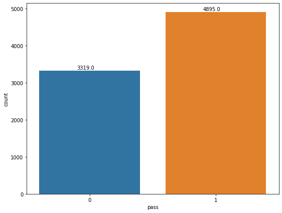
# Lets check if the movies pass bechdel test
li = []
for i in data_bechdel['Bechdel Score']:
  if(i<3):
    li.append(0)
  else:
    li.append(1)

data_bechdel['pass'] = li
data_bechdel.head()
data_bechdel['pass'].value_counts()
1    4895
0    3319
Name: pass, dtype: int64
figure(figsize=(9,7))
ax = sns.countplot(data=data_bechdel,x='pass')
for p in ax.patches:
   ax.annotate('{:.1f}'.format(p.get_height()), (p.get_x()+0.3, p.get_height()+40))
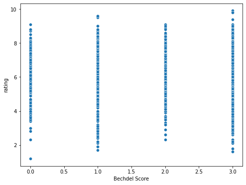
Lets Check the relationship between Imdb rating and bechdel scores
from pandas.core.reshape.merge import merge

url = r"https://raw.githubusercontent.com/Natassha/Bechdel-Test/master/movies.csv"
imdb = pd.read_csv(url,encoding='cp1252')
imdb.head()
imdbNew = imdb[['title','rating']]
imdbNew
(ggplot(data_bechdel)+geom_point(aes('year',color=data_bechdel['Bechdel Score']),stat='count',show_legend=False)+geom_line(aes('year',color=data_bechdel['Bechdel Score']),stat='count',show_legend=False))
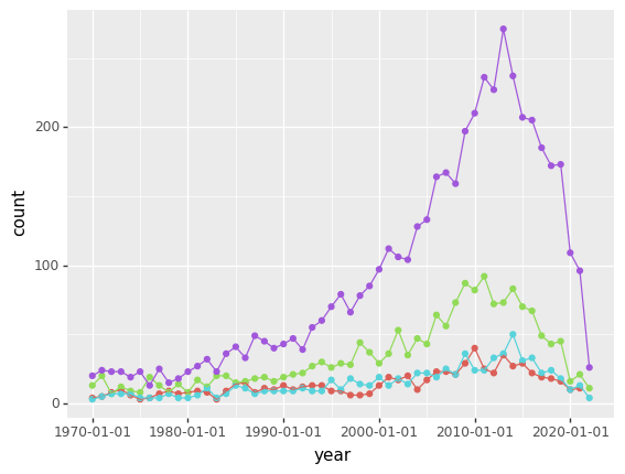
<ggplot: (8762740129624)>
data_bechdel = pd.merge(data_bechdel,imdbNew, how ='left',
                 left_on = ['title'], right_on = ['title'])
data_bechdel.head()
data_bechdel['rating'].value_counts().sort_index(ascending=False)
9.9    1
9.8    3
9.6    2
9.5    1
9.4    1
      ..
1.9    2
1.8    2
1.7    1
1.6    2
1.2    1
Name: rating, Length: 81, dtype: int64
figure(figsize=(8,6))
sns.scatterplot(x =data_bechdel['Bechdel Score'],
                y = data_bechdel['rating'],data=data_bechdel);
# Droping rows with null values
data_bechdel.dropna(inplace=True)
data_bechdel.drop('id',axis=1,inplace=True)
Creaing new dataframe with only year, bechdel score and rating
new = data_bechdel.groupby(['year','Bechdel Score']).agg({'rating':'mean'}).reset_index()
new.head()
| year | Bechdel Score | rating | |
|---|---|---|---|
| 0 | 1970-01-01 | 0 | 7.150000 |
| 1 | 1970-01-01 | 1 | 7.054545 |
| 2 | 1970-01-01 | 2 | 6.866667 |
| 3 | 1970-01-01 | 3 | 6.440000 |
| 4 | 1971-01-01 | 0 | 6.875000 |
Visualizing the relationship
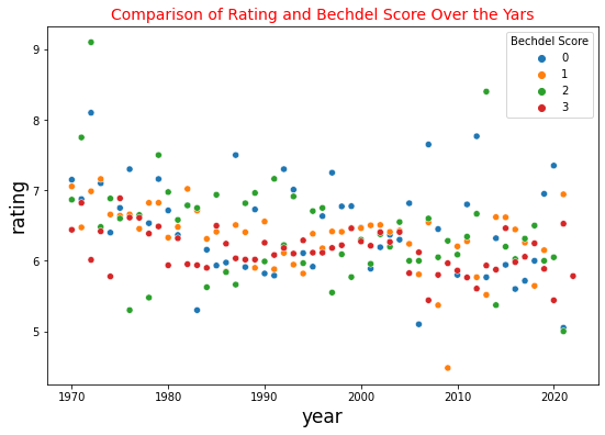
fig, ax = plt.subplots(figsize=(9, 6))
p = sns.scatterplot(x = 'year', y = 'rating',hue='Bechdel Score', data = new,ax=ax)
p.set_xlabel('year', fontsize = 17)
p.set_ylabel('rating', fontsize = 17)
p.set_title('Comparison of Rating and Bechdel Score Over the Yars', fontsize = 14, color='red');
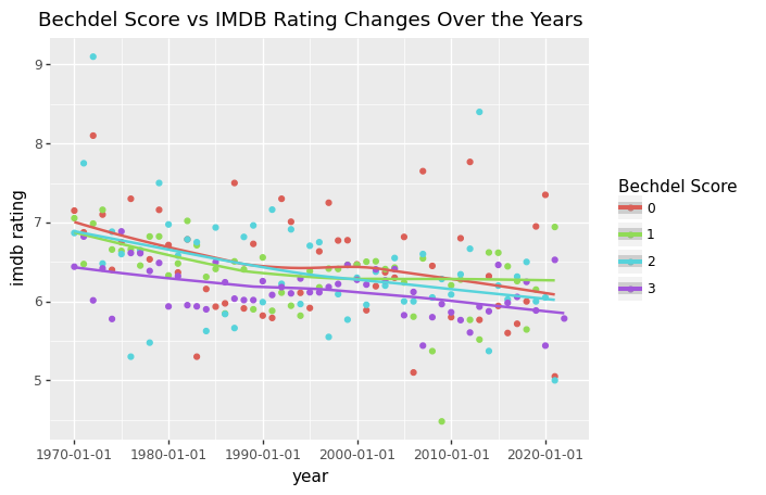
# Plot year against IMDB rating and Bechdel Score:
ggplot(new,aes(x='year',y='rating',color='Bechdel Score'))+ geom_point()+geom_smooth()+scale_y_continuous(name="imdb rating")+labs( colour='Bechdel Score' )+ ggtitle("Bechdel Score vs IMDB Rating Changes Over the Years")
<ggplot: (8762740129783)>
It appears as though movies that pass the Bechdel test have significantly lower IMDB ratings compared to movies that don’t, which was pretty surprising to me.
Now, I will try to visualize the relationship between the gender of the director and Bechdel scores. I assume that movies with female directors are more likely to have higher Bechdel scores, which I will try to plot here.
url = r"https://raw.githubusercontent.com/Natassha/Bechdel-Test/master/movielatest.csv"
latest = pd.read_csv(url,encoding='cp1252')
latest.head()
dfLatest = latest[['name','director']]
dfLatest.rename(columns={'name':'title'}, inplace=True)
data_combined = pd.merge(data_bechdel, dfLatest, how='left', left_on=['title'], right_on=['title'])
data_combined = data_combined.dropna()
data_combined.head()
| Bechdel Score | imdbid | year | title | pass | rating | director | |
|---|---|---|---|---|---|---|---|
| 35 | 1 | 0067800 | 1971-01-01 | Straw Dogs | 0 | 7.4 | Rod Lurie |
| 36 | 1 | 0067741 | 1971-01-01 | Shaft | 0 | 6.5 | John Singleton |
| 37 | 1 | 0067741 | 1971-01-01 | Shaft | 0 | 6.0 | John Singleton |
| 53 | 1 | 0067128 | 1971-01-01 | Get Carter | 0 | 7.4 | Stephen Kay |
| 54 | 1 | 0067128 | 1971-01-01 | Get Carter | 0 | 4.7 | Stephen Kay |
The newly created data frame now has an additional variable in it; director. I will now try to predict the gender of the director given their first name, and append it to the data frame.
# !pip install gender-guesser
import gender_guesser.detector as gen
# Predicting gender of director from first name:
d = gen.Detector()
genders = []
firstNames = data_combined['director'].str.split().str.get(0)
for i in firstNames[0:len(firstNames)]:
    if d.get_gender(i) == 'male':
        genders.append('male')
    elif d.get_gender(i) == 'female':
        genders.append('female')
    else:
        genders.append('unknown')
data_combined['gender'] = genders
data_combined = data_combined[data_combined['gender'] != 'unknown']
# Encode the variable gender into a new dataframe:
data_combined['Male'] = data_combined['gender'].map( {'male':1, 'female':0} )
data_combined.head()
| Bechdel Score | imdbid | year | title | pass | rating | director | gender | Male | |
|---|---|---|---|---|---|---|---|---|---|
| 35 | 1 | 0067800 | 1971-01-01 | Straw Dogs | 0 | 7.4 | Rod Lurie | male | 1 |
| 36 | 1 | 0067741 | 1971-01-01 | Shaft | 0 | 6.5 | John Singleton | male | 1 |
| 37 | 1 | 0067741 | 1971-01-01 | Shaft | 0 | 6.0 | John Singleton | male | 1 |
| 53 | 1 | 0067128 | 1971-01-01 | Get Carter | 0 | 7.4 | Stephen Kay | male | 1 |
| 54 | 1 | 0067128 | 1971-01-01 | Get Carter | 0 | 4.7 | Stephen Kay | male | 1 |
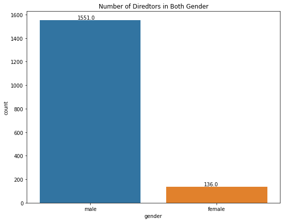
figure(figsize=(9,7))
ax = sns.countplot(x='gender',data= data_combined)

plt.title("Number of Diredtors in Both Gender")
for p in ax.patches:
    ax.annotate('{:.1f}'.format(p.get_height()), (p.get_x()+0.3, p.get_height()+10))
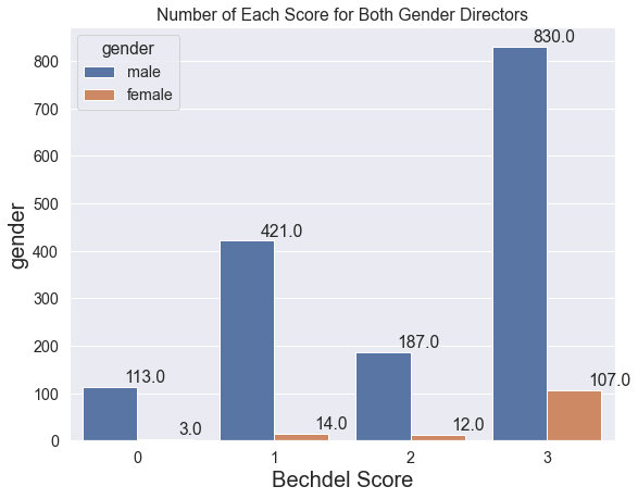
Next, I will visualize the gender of the director with the Bechdel score, to see if movies with female directors have a higher score.
sns.set(font_scale=1.3)
figure(figsize=(9,7))
ax = sns.countplot(x='Bechdel Score',hue='gender',data=data_combined)
ax.set_xlabel('Bechdel Score',fontsize=20)
ax.set_ylabel('gender',fontsize=20)
plt.title("Number of Each Score for Both Gender Directors")
for p in ax.patches:
    ax.annotate('{:.1f}'.format(p.get_height()), (p.get_x()+0.3, p.get_height()+10))
Next, I will take a look at the variable budget, to see if there is any kind of correlation between the budget of a movie and it’s Bechdel score.
data_combined['budget']=latest['budget']
ggplot(data_combined,aes(x = 'year', y ='budget' ,color='Bechdel Score'))+geom_point()+geom_smooth()+ ggtitle("Bechdel Score vs Budget Changes Over the Years")
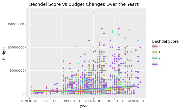
<ggplot: (8762740166012)>
Now, I will visualize the relationship between budget and gender of the director:
data_combined['budget']=latest['budget']
# Visualize budget and gender of director
ggplot(data_combined,aes(x = 'year', y = 'budget',color='gender'))+\
geom_point()+geom_smooth()+\
ggtitle("Bechdel Score vs Gender Changes Over the Years")

<ggplot: (8762622883904)>
data_combined['gross']=latest['gross']
ggplot(data_combined,aes(x = 'year', y = 'gross',color='gender'))+geom_point()+ ggtitle("Gross Revenue vs Director Gender Changes Over the Years")

<ggplot: (8762724703166)>
From the above analysis, it can be observed that number of movies that pass the Bedchel test has been increased. Another result is that female directors have positive impact on movies Bedchel test performance. Although the Bedchel test is well-known test, it is not best one to make conclusion about the movies since there different parameters that need to be taken in consideration.